Author: Daniel Zhang

Important

Click Use this template button (NOT fork) to create your repo based on it

Warning

Do not modify the provided debug preset in CMakePresets.json, as it may cause CI (GitHub Actions) failure. Add your own preset instead if you don't want to use the provided one.

Rules

• You may use any course material, including this lab's prep material, its solution, and the C++ notes, without citation.
• Check the appropriate preconditions and postconditions. Your program should not crash or have undefined behaviour (hint: use assertions).
• Test all implemented code. Use your compiler's address sanitizer (g++ flag -fsanitize=address), or tools such as valgrind and leaks, to check for memory leaks.
• Your programs must be well structured and documented. Use Ctrl-X T in Emacs to pretty-print them. Marks are assigned for functionality, program appearance, and comments.
• If your program hangs, use Ctrl-C to terminate it.
• Include the appropriate header files. To find which headers you need for functions such as printf, use the man command.

Problems

1. Row- vs. Column-major Traversal Order

In p1.cpp, allocate two separate contiguous arrays of uint64_ts, each of size 16,000,000. Treat both as 2D arrays of size $4000 \times 4000$. You may also allocate two 2D arrays directly on the heap, but each must be contiguous.

Use the 64-bit Mersenne Twister with a seed of 0 to fill both arrays with exactly the same random values, but in different orders:

• Fill the first in row-major order: the outer loop iterates over row indices.
• Fill the second in column-major order: the outer loop iterates over column indices.

Time, in microseconds, how long it takes to sum the first array into a uint64_t, again in row-major order. Then time how long it takes to sum the second array into a uint64_t, in column-major order. Both sums should iterate over the exact same numbers in the same sequential order, but with a different memory access pattern. The sums should therefore be the same; you can ignore overflow.

Your program should print two lines. First, print the time the first array took to sum, followed by a space and the sum. The second line has the same format for the array traversed in column-major order.

Example output, with made-up sums, if both sums took 50 milliseconds:

50000 19238427384827342
50000 19238427384827342

Ensure your program does not leak memory. It must compile without errors or warnings with cmake --build release.

In p1.txt, report your results (the program's output) and justify the timings in 1–2 sentences.

2a. Space-filling Curves

In this part, implement a space-filling curve known as the Z-order curve, also called the Morton code, Morton order, or Lebesgue curve. Morton codes order high-dimensional points so that nearby points in space tend to be close in the one-dimensional ordering.

Z-order Curves

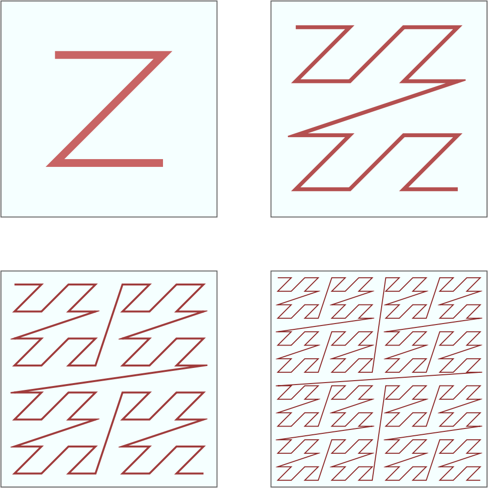
Z-order curves

David Eppstein

Two-dimensional Z-order curves for k = 1, 2, 3, 4. Traversal starts at the top-left and follows the line to the bottom-right.

Setup

The Morton curve has two hyperparameters:

1. The dimensionality of the space, $d \in \mathbb{N}$.
2. The integer $\log_2$ of the number of discrete values along each dimension, $k \in \mathbb{N}$. For example, if $k = 4$, imagine a ruler along each axis with $2^k = 2^4 = 16$ discrete points.

Given $d$ and $k$, define a $d$-dimensional space of $(2^k)^d = 2^{kd}$ distinct points, with each axis having values in $\{0, \dots, 2^k - 1\}$. A point in this space is identified by its coordinates:

$$\mathbf{a} = (a_1, \dots, a_d)$$

where $a_i \in \{0, \dots, 2^k - 1\}$ for $1 \leq i \leq d$. Each $a_i$ can be stored in $k$ bits, denoted by:

$$a_i = 0ba_{i,k-1}a_{i,k-2}\dots a_{i,0}$$

The $0b$ prefix indicates binary, as it does in C++. Each $a_{i,j} \in \{0, 1\}$, and $a_i = \sum_{j=0}^{k-1} a_{i,j}2^j$.

Given coordinates $\mathbf{a} \in \{0, \dots, 2^k - 1\}^d$, the Morton code maps them to a single integer position $\mathrm{morton} (\mathbf{a}) \in \{0, \dots, 2^{kd} - 1\}$ by interleaving the bits of each coordinate $a_i$.

Examples

Before the formal definition, consider a 2D $4 \times 4$ space: $d = 2$, $k = 2$, corresponding to the top-right curve in the diagram. One point is $(1, 3) = (0b\underline{01}, 0b11)$. Its Morton order index is $0b1\underline{0}1\underline{1}$, where the underlined bits came from the first coordinate dimension, $a_1$.

For $d = 2$ and $k = 4$:

$$\mathrm{morton} (0b\underline{0000}, 0b1111) = 0b1\underline{0}1\underline{0}1\underline{0}1\underline{0}$$

In 3D, for $d = 3$ and $k = 4$:

$$\mathrm{morton} (0b\underline{0001}, 0b0010, 0b\overline{0100}) = 0b\overline{0}0\underline{0}\overline{1}0\underline{0}\overline{0}1\underline{0}\overline{0}0\underline{1}$$

Formal Definition

The Morton code of a coordinate $\mathbf{a} \in \{0, \dots, 2^k - 1\}^d$ is:

$$\mathrm{morton} (\mathbf{a}) = 0ba_{d,k-1}a_{d-1,k-1}\dots a_{1,k-1}\dots a_{d,0}a_{d-1,0}\dots a_{1,0}$$

Implementation

In p2a.h, implement:

inline uint64_t morton3d(uint64_t x, uint64_t y, uint64_t z)

This implements the Morton code for $d = 3$ and $k = 64$, where $x := a_1$, $y := a_2$, and $z := a_3$. Truncate the bits of the true output at bit index 64 and greater. Your implementation must run in $O (\text{word size})$ time and require at most $O (1)$ words of space.

Reuse expand

Use expand from the prep. Since it will now be implemented in a header file, mark it inline to avoid a One Definition Rule violation if the same header is included in multiple files.

2b. Memory Layout of Higher-dimensional Arrays

In p2b.cpp, write a C++ program that implements, tests, and times convolution of two heap-allocated contiguous 3D arrays in these layouts:

• $A$: Standard (row-major) order, as an array of $Z$ arrays of $Y$ arrays of $X$ uint64_ts.
• $B$: Morton order, as defined in part 2a, also containing uint64_ts.

Representing the Morton-order array

It is easiest to represent the second array as a 1D array of length $Z \times Y \times X$ and index into it using morton3d(x, y, z) from part 2a.

Use the shape $(X, Y, Z) = (256, 256, 256)$, for which $X \times Y \times Z = 16777216$. Randomly initialize the elements of the row-major array $A$ in the order they are laid out in memory, using a 64-bit Mersenne Twister seeded with 0. Then copy $A$ into $B$ in Morton order so that they represent the same array with different memory layouts:

B[morton3d(x, y, z)] = A[rowMajorIndexA(x, y, z)];

Do this for every valid $x$, $y$, and $z$. If you represent $A$ directly as a 3D array, the right-hand side will look slightly different.

Convolution

If you are already familiar with convolutions, use a kernel $K$ of shape $4 \times 4 \times 4$, a stride of 4, and no padding.

Intuitively, convolution takes two multidimensional arrays and slides the smaller one within the larger one. At each position, take a dot product between the overlapping entries of the two arrays; this gives the value in the output array.

The stride is how far the smaller array slides along each dimension. It defaults to 1 in each dimension unless otherwise specified. The padding is the number of extra pixels or voxels added to the edges of the larger array to obtain a particular output size. Padding is not needed in this exercise.

For a 2D example, consider a kernel $K$ of shape $2 \times 2$ and a matrix $M$ of shape $4 \times 4$, with lines added as a visual guide:

$$\begin{aligned} M &= \left[\begin{array}{cc|cc} 1 & 2 & 3 & 4 \\ 5 & 6 & 7 & 8 \\ \hline 9 & 10 & 11 & 12 \\ 13 & 14 & 15 & 16 \end{array}\right] & K &= \begin{bmatrix} 0 & 1 \\ 2 & 0 \end{bmatrix} \end{aligned}$$

The convolution of $K$ over $M$ with stride 2, denoted $M * K$, is:

$$M * K = \left[\begin{array}{c|c} 12 & 18 \\ \hline 36 & 42 \end{array}\right]$$

Start with $K$ overlapping the top-left corner of $M$. The dot product of the overlapping entries is $(1 \times 0) + (2 \times 1) + (5 \times 2) + (6 \times 0) = 12$, the top-left result. For each position $(x, y)$ in $M * K$, shift $K$ to $2x$ and $2y$ (because the stride is 2) and repeat the computation. Here, the result has shape $(X/2, Y/2) = (2, 2)$.

In 3D, slide the smaller 3D array along each of the three dimensions. For an input $M$ of shape $(X, Y, Z)$ and a kernel $K$ of shape $(1, 2, 3)$, no padding and a stride of 1 in each dimension give an output of shape $(X, Y - 1, Z - 2)$. With a stride of 2 in each dimension, the output shape is:

$$\left (\left\lfloor\frac{X - 1}{2}\right\rfloor + 1, \left\lfloor\frac{Y - 2}{2}\right\rfloor + 1, \left\lfloor\frac{Z - 3}{2}\right\rfloor + 1 \right)$$

In general, along dimension $i$, let the padding be $P_i$, the stride be $S_i$, the input length be $|M|_i$, and the kernel length be $|K|_i$. The corresponding output length is:

$$|M * K|_i = \left\lfloor\frac{ (|M|_i + 2P_i) - |K|_i}{S_i}\right\rfloor + 1$$

Implementation and Timing

Store your $4 \times 4 \times 4$ kernel wherever you please, initialized with $K (x, y, z) = x + y + z$ for $0 \leq x, y, z < 4$. Make two versions: $K_a$ in row-major order and $K_b$ in Morton order.

Fully convolve $K_a$ over $A$ into a row-major 3D array on the heap, then convolve $K_b$ over $B$ into a Morton-order 3D array on the heap. Use no padding and a stride of 4 along each dimension.

Use Timer from the prep to measure the runtime of each convolution. Print the times in microseconds, one per line. Do not print the convolution results, but do assert that every output entry in $A * K_a$ equals the equivalent entry in $B * K_b$.

In p2b.txt, report your results and justify them in 1–2 sentences.

Ensure your program does not leak memory. Use your compiler's leak sanitizer or tools such as valgrind to check. Your program must compile without warnings with -Wall -Wextra -Wpedantic. For timing, you may add -DNDEBUG to turn off assertions once you are confident your code is correct.

Hint 1: Row-major indexing

If you represent $A$ as a 1D array, you may wish to write three helpers to index into $A$, $K_a$, and $A * K_a$:

size_t rowMajorIndexA(size_t x, size_t y, size_t z)
size_t rowMajorIndexK(size_t x, size_t y, size_t z)
size_t rowMajorIndexConv(size_t x, size_t y, size_t z)

These necessarily differ because the three 3D arrays have different shapes. This is unnecessary for the Morton index: its computation is the same regardless of the array shape, so long as the space has a side length that is a power of two.

Hint 2: Row-major convolution

Convolution over the row-major array $A$ may involve a six-level nested loop.

Hint 3: Morton-order convolution

Convolution over the Morton-order array $B$ can be simplified to a double-nested loop. Refer to the Z-order diagram and consider how each consecutive subdivided block of shape $4 \times 4 \times 4$ is laid out in memory. As $k$ increases, the previous level is recursively and consecutively embedded in it. Do you need any calls to morton3d to take the dot product if both $K_b$ and each $4 \times 4 \times 4$ block in $B$ are laid out the same way?